By Suddhasatwa Bhaumik.Oct 30, 2022

Motivation
Hello Readers!
What follows is a series of Blog posts about BigQuery (and related products in GCP, including BigLake, Omni, et al) covering in depth information about its design, architecture, working and best practices.
Here’s a small index of the parts of this Blog post (which will be kept updated from time to time as new parts of the series are written):
- Part # 1 — Introduction, Basics of BigQuery, and BigQuery Architecture
- Part # 2 — BigQuery Storage, Design Principles & (Some) Best Practices
Introduction
BigQuery is the flagship Data Warehousing and Data Analytics product of Google Cloud Platform (GCP). Out of its in-numerous use cases and applications, the basic ideology behind this technology is to provide GCP customers with an easy to use SQL based interface from GUI (Graphical User Interface, a.k.a. the GCP Console) or the CLI (Command Line Interface, or the GCP SDK) to perform Data Warehousing tasks at scale!
In this post, we will revisit the basics of Data Warehousing concepts, followed by the basics and internal working details of BigQuery. In the upcoming parts of this series of blog posts on BigQuery, we will cover other aspects of the software, including BigLake, BigQuery Omni, Machine Learning Capabilities, and so on.
Basics Of Data-warehousing
Before knowing in detail about BigQuery, it’s crucial that we all revise the common terminologies. Most of us are already well versed with this, but there is nothing wrong in a revision!
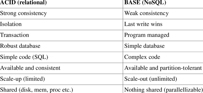
In any organisation or setup, the available data can be collected and then stored in different places with different technologies or different methodologies! Often, we reuse the term database to reference a transactional system where we may store the data generated by an application or system. By design, it is optimised to efficiently retrieve and update information. These databases can be either SQL or No-SQL databases, depending on their design and normalisation properties. Part of the Google Cloud Platform suite of databases, the list of such databases include BigTable, Spanner, Cloud SQL, and so on. There are different ways in which these transaction databases incorporate ACID or BASE principles respectively.
Once we had the invent of Traditional database systems, there was an inherent need of analysing massive sets of data stored in these systems by their respective applications. But, there is a problem!
These transactional systems are not optimised by design for performing large scale analytics by default, because they inherently contain the notions of normalised tables in many cases, resulting into joins, and hence inefficiency at scale!
This brings us to the advent of Data Warehouses and the great era of possibilities the latter offers for large scale Data Analytics and Data Science applications.
In simple terms:
A Data-warehouse stores information from a variety of data sources for Analysis purposes, with an inherent design that supports such operations, even at scale!
It was until the recent years, that we have also come up with concepts of Data Marts and Data Lakes, which may have different definitions to different people, depending on the relevant understanding and the use cases they solve.
For the context of this article, let’s put things in simple words:
- A Data Lake is a data dump yard — this is where we store all RAW files, often containing Unstructured data, and acts as a staging environment, before the transformed and cleaned extracts of data is put into Data warehouses!
- A Data Mart is a segment/part of a data warehouse — which is designed specifically for something or someone very specific, like a department in our organisation!
Keeping above revision in mind, let’s now deep dive into BigQuery.
BigQuery — Query Big Data!
As the most prominent Data Analytics product of Google Cloud Platform, BigQuery is a perfect solution of a Data warehouse, which also supports implementations of Data Lakes and Data Marts! In this way, it brings the best of all the OLAP (Online Analytical Processing) requirements of an Analytics Platform, relieving us from the limitations of Data Analytics on OLTP (Online Transaction Processing) Database Systems.
For many, however, the definition of BigQuery can be suitably different depending on our role and how we perceive it!
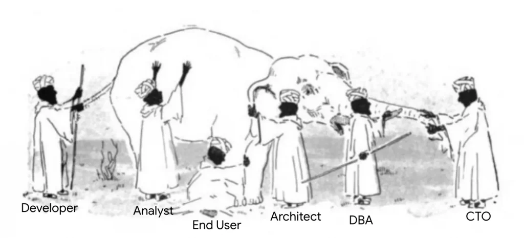
The ideation of BigQuery started actually from the ground concepts of Map Reduce Programming Model in reality! To quickly revise:
MapReduce is a programming model and an associated implementation for processing and generating big data sets with a parallel, distributed algorithm on a cluster.[1][2][3]
A MapReduce program is composed of a map procedure, which performs filtering and sorting (such as sorting students by first name into queues, one queue for each name), and a reduce method, which performs a summary operation (such as counting the number of students in each queue, yielding name frequencies). The “MapReduce System” (also called “infrastructure” or “framework”) orchestrates the processing by marshalling the distributed servers, running the various tasks in parallel, managing all communications and data transfers between the various parts of the system, and providing for redundancy and fault tolerance.
Reference: https://en.wikipedia.org/wiki/MapReduce
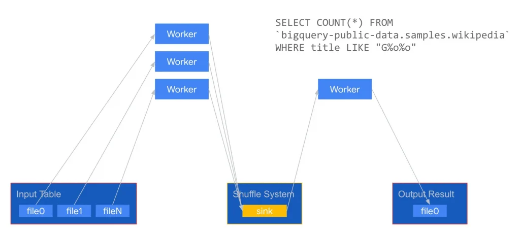
Interestingly, this is exactly what BigQuery does (or, at least tries to do) under the hood! Before even looking at its detailed organisation or architecture details, let’s quickly understand how a typical query gets executed in BigQuery in a simple way:
Essentially, for every query ran on BigQuery we have a map stage (the first square box on bottom left corner, and the next one with Workers), where the data is mapped to specific workers, and maybe filtered or sorted depending on the query syntax and semantics. Further, the resulting subset of the data is written out to some intermediate stage (mentioned above, as the Shuffle System), and then finally, reduced in the final stage (by the Worker in the above diagram), so that the output can be written out the user (in form of an Output Result Object). Although we go in depth of query execution in later parts of this series of posts, it is interesting to note couple of points above:
- The input or data at rest is seen to be chunked or divided into parts.
- Each worker in the initial stage handle one specific part of the data.
- All are brought in together for Shuffle stage at once.
- Finally the result is output by one (or more) workers to the Disk.
For above to work effectively, we need substantial improvements over how we used to execute Map Reduce programs in known frameworks like Hadoop. A couple of them, along with the solution which BigQuery uses in the background are:
- a highly scalable and high throughput network: this is where Google’s super-fast and global scale petabyte scale network Jupiter comes to play!
- a highly redundant and performant disk organisation: this is where Colossus comes to rescue!
- a sophisticated processing engine, which can improve the program execution using techniques like Vectorisation: this is where Dremel comes to play!
Above example (in the diagram) had a mediocre query; in case of large scale joins and bigger executions, the overall strategy followed within BigQuery can be summarised in the following picture:
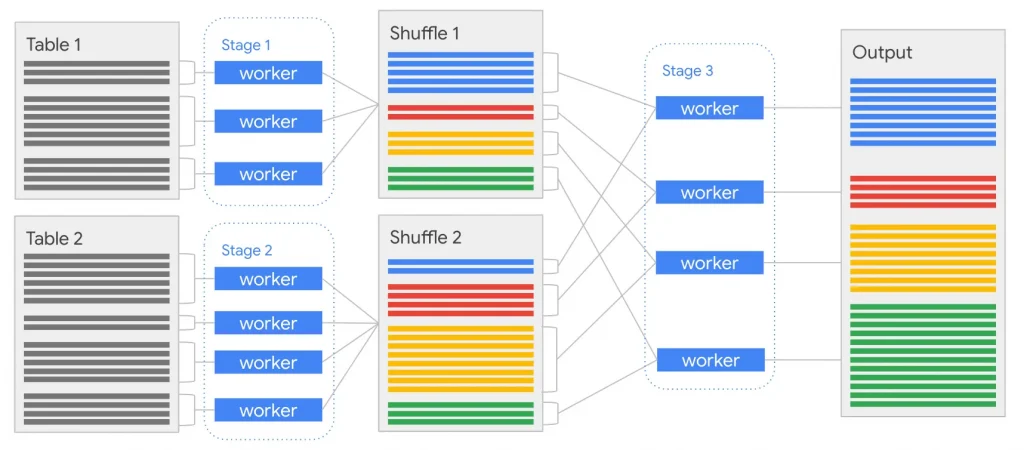
In summary, for a large scale join, first the data is mapped to workers, wherein they are basically just reading from the distributed storage, and then the data is sorted so that the rows for each hash of the join key end up in the same worker!
Now, let us gently understand BigQuery’s architecture.
BigQuery Architecture — A Gentle Introduction
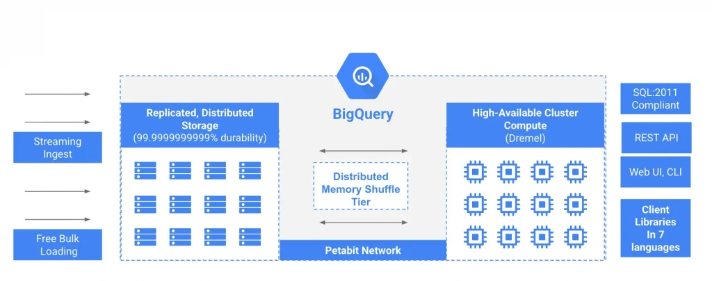
Let’s explore the above pictorial representation of the overall architecture of BigQuery point by point:
- Firstly, we need to note that, storage and compute are separate and are scaled independently and on-demand. This is the essence of BigQuery’s excellent performance for Large Scale data analysis use cases!
- Within the middle block of architecture, we meet Colossus — Google’s Distributed file system, this is where BigQuery natively stores customer data in Google Cloud Platform. On the right side of the architecture, we find Dremel, our Query engine!
- Comparing to traditional transactional databases, the storage and compute units in the former are natively stored very close to each other to guarantee ACID principles as well as for Performance. As of date, we have larger networks that are remarkably fast, hence tight coupling is no longer a hard-bound! Again, we plan to practice really large scale analytics, and hence, the queries are often running for a while to process all our data! This means, latency is also not as important.
In case of BigQuery, decoupling storage and compute has substantial benefits, like following:
- Scalability: Without any data movement, new nodes can be added to the cluster of nodes! Therefore, scaling out a cluster with separated compute and storage is very fast (I.e., in terms of few seconds), as compared to hours or days for databases where compute and storage is tightly coupled.
- Availability: In case of node failures, the data is never lost! The surviving nodes in the cluster can access all data (through the network), hence any or all system recoveries from node failure is performed very quickly, by one (or more) of the surviving workers!
In the middle of the above architecture diagram, we also have the distributed memory shuffle, which we will surely deep dive in the upcoming posts. All of these operations are running on Jupiter, Google’s huge petabyte scale network, which allows anyone of the Google Cloud Platform customers to efficiently take advantage of Google’s scale as an organisation.
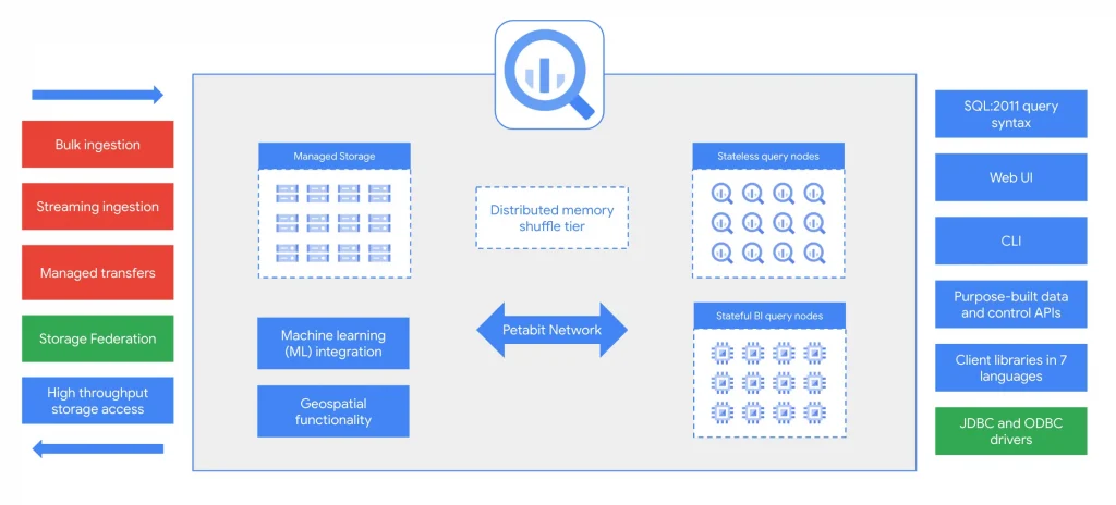
Other than the basic design principles, we also find that:
- There are plethora of methods by which we can ingest data into BigQuery for Analytics. Most common methods include Batch/Bulk ingestions using Command Line or other GCP Products like Dataflow, Streaming ingestions using BigQuery Streaming options or Dataflow, Managed transfers using BigQuery Data Transfer Service option, to name a few.
- Storage federation option is in-built into BigQuery as a service, so that we can conceptualise our data lake even in Google Cloud Storage and read (usually structured or JSON/XML) data directly in form of hypothetical external tables in BigQuery.
- To interact with BigQuery programmatically, like a Data Analyst, not only do we have standard SQL dialect, but we also have machine learning integration, and features like geospatial functionality.
- By design in BigQuery, we have stateless worker nodes. In simple terms, these are our standard compute workers to execute queries. Additionally, as of date, we also have the BI query nodes, for BI engine, where queries are executed in-memory to make things super fast. More of BI Engine later!
- We can also interact with BigQuery through the Web UI, Command Line interface, client libraries etc. This makes BigQuery extremely flexible for developers, only limited by the different user personas enacted by IAM Roles.
Conclusion: Part # 1
Hope this first set of introduction to BigQuery and its internals is useful to our readers (data engineers, data scientists, alike!). In the next parts of this series of Blog posts, we will uncover more internal working of BigQuery, starting with how the Storage (Colossus) works internally, how the Dremel query execution engine efficiently runs our queries, and so on.
For our readers who are looking for a quick introduction over Video format, there is already an excellent playlist created by our fellow Googlers in Youtube! It is available here.
Happy learning!!!
The original article published on Medium.


