By Suddhasatwa Bhaumik.Nov 1, 2022
Introduction
In the first post of this series of posts, available here, we have seen the basics of BigQuery and how it “fits” into the Data Analytics and Data Science ecosystem of Google Cloud Platform for all our customers, by being a Data warehouse with Analytics and Machine Learning Capabilities on Google scale of data, available for all our customers of Google Cloud Platform!
In this blog post, we will discuss and learn about how the back-end is designed in BigQuery for storage, specifically the Colossus File system, how it works internally, and how we can make the best use of Storage by using methods of Partitioning and Clustering, and other tips!
Storage Under The Hood!
Under the hood, BigQuery uses Colossus for storage of data. Deep inside Colossus, though, it uses Capacitors! Let’s understand what a Capacitor really is, by firstly understanding how a traditional database system is designed to handle data storage.
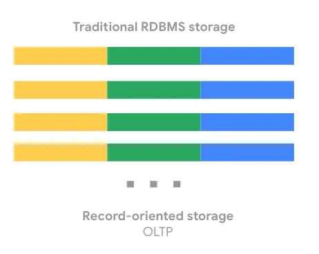
Traditional Relational Databases, like Postgres or MySQL, by design, store data row-by-row (a.k.a., record-oriented storage). This makes them really efficient for online transactional updates or OLTP use cases! On Google Cloud Platform (GCP), we make use of Cloud SQL (our managed database solution offering) for a large amount of transactional updates. Overall the organisation of data looks like below:
BigQuery, on the other hand, uses columnar storage, where each column is stored in a separate area on the residing disk. The chunk of data stored on disks is otherwise fondly known as Capacitors. In simple words, capacitor is the file format of storage on Colossus system for BigQuery data. More on how to load data, later!
Meanwhile, if we think about queries that developers and analysts write and execute against OLTP (transactional) databases (like Oracle and MySQL), storing the data row by row is more sensible, not only because the database needs to adhere to the ACID principles but also because it is used more for bulk writes and selective reads on Row levels, usually, although there are variations to this statement in the way we have seen customers using their OLTP databases. E.g., there are indeed large corporations worldwide who effectively make use of Oracle database, as an example, for all of their OLTP and OLAP use cases by proper indexing of the data and by creating aggregation layers for reporting and analytical use cases.
However, if we have analytical use cases, (like, for example) wherein, we would want to calculate the average age of our followers on Facebook, the data engineer or analyst, working on this use case, would need to read in all the information about every single person !! In case our data is stored in Row storage format, now this overall operation would be really inefficient, since we will end up reading almost all of the rows!
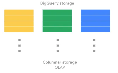
Instead, with columnar oriented storage, like what we have in BigQuery in form of Capacitors, we can just read in the specific “age” column!
Important Note: Remember, this is the basic reason why a SELECT * is the MOST DANGEROUS operation in BigQuery. It is not only performance unfriendly but also incurs humongous amount of costs while operating on a BigQuery dataset. More on Datasets, later!
Now, let’s dig deeper into Capacitor and its design/working!
Mr. Capacitor!
Overall, the below diagrammatic representation provides an overview of how the Capacitor file format is used to store data in chunks on columnar levels of storage in Colossus.
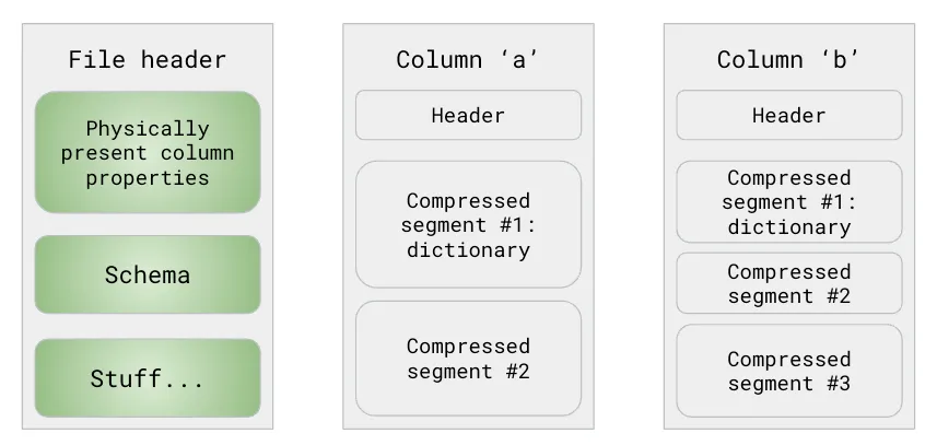
As defined, Capacitor is a column-oriented format — this means, the values of each field are stored separately, so the overall I/O overhead (during any or all of the read and write operations) is proportional to the number of fields you actually read! However, this doesn’t necessarily indicate, that each column is in its own file; it simply designates that each column is stored in a file block, which is further compressed independently.
Capacitors are also self-describing, so the information in the file itself is always sufficient to fully decode and read it. This is made possible by the component, called File Header, as seen in the above diagram.
The so-called File Header contains all the metadata related details about columns present in the file. This includes, but obviously not limited to, the column name, data type, and other metadata details, for each and every column. Each column also has min/max, which may be used from time to time by the BigQuery query execution engine, a.k.a Dremel, to arguably reject the entire file. More on the execution of queries in BigQuery is to be covered in later posts!
Further, each column also has compressed information — in essence, BigQuery uses different encodings to optimise storage. This makes a huge performance benefactor while related business filtering conditions are applied on top of columns during read operations!
Now, let’s quickly look at some examples of how data encoding is done by BigQuery, all by itself! What follows now, is by no means a definitive list of all possible methods of encoding, but only a handful for example purposes.
Encoding Of Column Data
One common way of encoding column data, as used by BigQuery, is Dictionary based Encoding, an example of which is shown below:
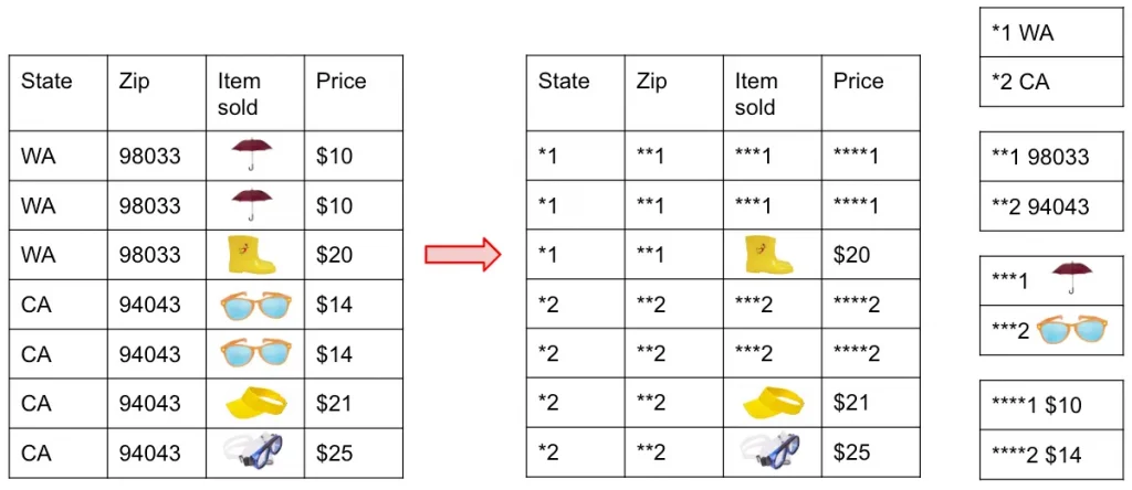
What is effectively happening is the way the original data, shown on the left side of the above diagram, is being stored internally as organised like a dictionary, as shown on the right side of the diagram!
Also known as Run length encoding method, this allows BigQuery to efficiently store repeated values, so instead of saying *1 three times, BigQuery would just record that it is repeated three times.
Another very common approach to consider is Record Reordering which is also another way of how BigQuery organises the data internally for faster analytical operations.
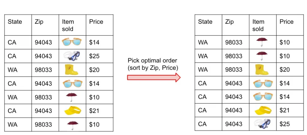
Essentially, what is happening here is, Capacitor is internally re-ordering records, to be able to try and group repeated fields, so as to make Run Length Encoding (RLE) method more successful!
Before we move over to best practice based design patterns in BigQuery, let’s conclude the storage aspect of BigQuery by finally understanding the actual physical storage layout in simple terms in lieu of Colossus system.
Colossus: Physical Storage Pattern
Overall, the Colossus File system looks like the diagram below:
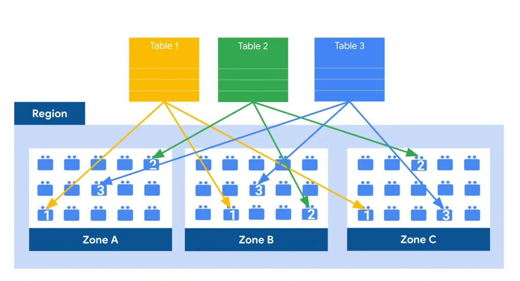
Overall, and as seen above, BigQuery storage is a Regional &/or Multi-Regional service, as chosen during creation of a “dataset” (I.e., synonymous to Schemas in OLTP Databases, more on that later!). With one region in GCP being sub-divided into multiple zones, hence each “table” (one single logical entity of data in BigQuery, just like any other database!) is replicated across multiple Regions for failover scenarios, when the dataset to which the table belongs is created using a Regional option.
By design, in Colossus,
- all data is automatically compressed, encrypted, replicated, and distributed.
- There are many levels of defence against unauthorised access in Google Cloud Platform, as we are aware of, wherein one of them is the fact that100% of data is encrypted at rest.
- Colossus ensures durability using erasure encoding to store redundant chunks of data on multiple physical disks.
Immediately upon writing data to Colossus, BigQuery starts the geo-replication process, mirroring all the data into different data centres around the specified region, in case the dataset to which the table belongs to is Regional.
Some critical points to be taken into account are as follows:
- In a single region, data is stored only in the region. Note: In this case, there is no Google Cloud–provided backup or replication to another region.
- In the event of a machine-level failure, BigQuery will continue running with no more than a few milliseconds delay. By design, all queries should still succeed. In the event of a zonal failure, no data loss is expected.
- Soft zonal failure, such as resulting from a power outage, destroyed transformer, or network partition, is already a well-tested path, as part of all the DR scenarios for BigQuery, which are regularly and thoroughly checked by our Engineering &/or SRE Team(s).
- If, unfortunately, a hard regional failure occurs by any reason, say, if any natural or unnatural disaster destroys the region, data in that region might be lost, if the dataset was created as a Regional dataset.
- A soft regional failure, on the other hand, will result in loss of availability, until the region is brought back online, but it will not result in lost data.
A multi-region location (in terms of Google Cloud Platform) is a large geographic area, such as the United States (US) or Europe (EU), that contains two or more geographic places.
- In a multi-regional type of dataset in BigQuery, data is stored in a single region but is backed up in a geographically-separated region to provide resilience to a regional disaster.
- The recovery and failover process is entirely and efficiently managed automatically by BigQuery.
Note: Many customers store their data in multi-regional datasets to ensure automated backups and better disaster recovery, but sometimes it is a better option, even from a legal or data privacy standpoint, to chose a single region for a dataset in BigQuery, which is aimed to be close to on-premise or to GCP Application workloads; this is done to minimise any latency between the Application and the BigQuery instances/workers!
Now, let’s carry over to some important design patterns in BigQuery which is also used for improving Analytical workload’s performance.
Design Patterns — Partitioning & Clustering !
The first and most important design pattern of BigQuery is Partitioning. When we (Data Engineers) design data warehousing solutions, it is often a best practice to partition our data basis the access patterns of the expected queries on top of our OLAP Database System. This improves the performance and scalability of the system upfront, and also helps to reduce maintenance over-head over time!
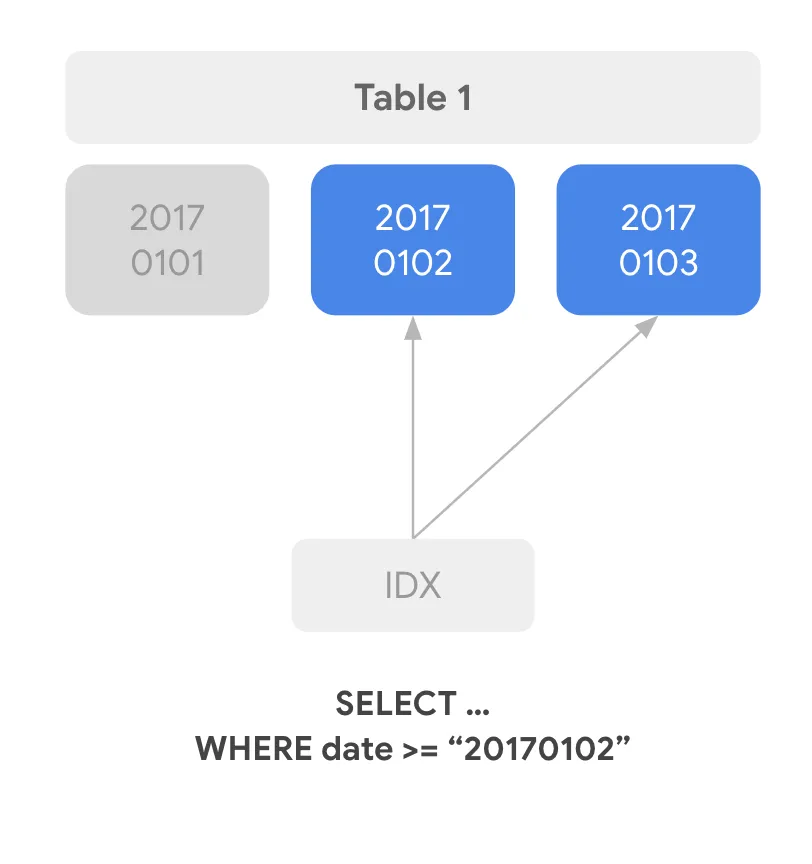
In BigQuery, too, data engineers and analysts often are encouraged to rely on partitioning the data stored in tables for appropriate levels of performance; this ensures that basis the filtering conditions only the selected partitions of data are queried rather than the entirety of it, hence reducing query execution time and cost.
But, how does partitioning (or pruning) actually work?
For Read Operations:
- Dremel, the BigQuery query execution engine, sends request to metadata server, which queries Storage Sets table (just another name for storage object on Colossus) filtering on the PartitionKey column (as mentioned in the WHERE clause), and finally, responds with the list of storage sets with PartitionKey within the requested range. This is not the actual data reading stage, but simply the data identification stage, as we can call.
- Next, Dremel opens capacitor files within StorageSets, checks the minimum & maximum values for each column in the file (available in capacitor file header, remember!).
- If [min, max] is outside the relevant range it will skip the remaining of the file, else data will be read from this file!
For Write Operations:
- Metadata from those storage files will be used to determine which fragments will be relevant.
- Rest of the update operations are almost exactly similar to Read operations!
There are 2 types of Partitioning possible on any BigQuery table:
- Ingestion date/time partitioning: Based on date/time that data is loaded. For this, we filter our table’s data using pseudo-columns: _PARTITIONDATE, _PARTITIONTIME. One example query can be: SELECT col FROM d.t WHERE _PARTITIONDATE > “2018–05–01”
- Column partitioning: Partition tables based on any of the following column types: TIMESTAMP, DATE, DATETIME (hour, day, month, or year granularity), INT64 (you define the range: start, end, and interval). Here again, we filter using column name and reduce data scanned. Example: SELECT COUNT(*) FROM d.t WHERE datecol > “2018–05–01”
Similar to Partitioning, another very important design pattern in BigQuery is Clustering wherein based upon the contents of up to 4 columns, the data in any given BigQuery table is sorted either automatically or by choice of data engineers!
However, below are a few points to be noted always about Clustering:
- Partitioning is not a requirement to cluster tables! We should avoid partitioning if table partition sizes are less than 1 GB.
- Yes — Clustering does result into Faster Queries because very less data scanned by only scanning relevant blocks of the data (in form of clusters) rather than the entire table.
- Certain queries leverage clustering for faster JOINs.
- Clustering is a pretty less expensive operation for BigQuery since proper filtering of data (based on clustered columns) reduces cost while improving performance.
- Lastly, clustering also prevents cost explosion due to user accidentally querying really large tables in entirety
Note: Many of our readers will be surprised to know that, BigQuery also performs Automatic Re-clustering of tables as a background task from time to time to inherently order the data in the tables.
Adaptive File Sizing
One of the less known but greatly beneficial design feature of BigQuery is that, out of the box it provides Adaptive File Sizing functionality!
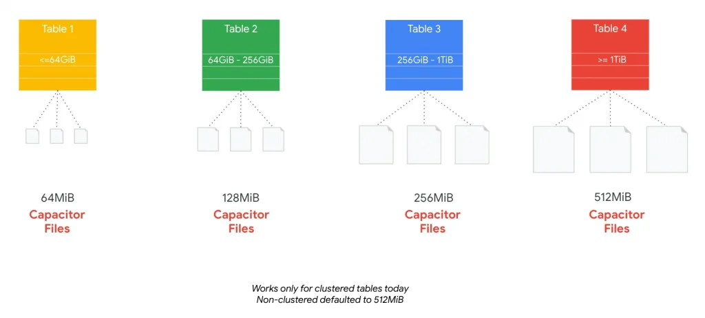
Note: as of the time of writing this post, only Clustered tables are supported or chosen for Automatic Adaptive File sizing, while the rest of the non-clustered tables/data in our BigQuery installation will default to a block size of 512MB.
However, for Clustered tables, BigQuery automatically adjusts the block size of the data, based on the size of the table, to allow for efficient queries over smaller datasets!
Remember: By design, BigQuery is tuned for throughput, rather than latency!
Ending Note
In this post, we have learnt quite a few things in relevant depth.
As an ending note, it is good to mention, that more often that not, a proper and well designed combination of Partitioning and Clustering (used together) can immensely improve the performance of the queries, provided the access patterns of our queries are supposed to benefit from grouping and ordering of underlying data at the first place.
Hence the decision to make the best use of Partitioning &/or Clustering should not be a mandate, but rather, it should be dominated by the queries intended to be run on our BigQuery setup for Analytical use cases.
In the upcoming post(s), we will cover further details about how BigQuery installations are organised for any customer project (typically), and optionally, we will later cover some use cases of BigQuery migration topics.
Happy Learning!!!
The original article published on Medium.

在〈BigQuery: Basics & Internals: Part # 2〉中有 1 則留言
cvs cialis cost
cvs cialis cost